An important feature of MLwiN is its graphical interfaces. These allow the user easily to set up, fit and manipulate models. There are windows for data manipulation, plotting, viewing the progress of iterations etc. Predictions from fitted models can be specified directly using standard statistical notation with direct links to various kinds of derived graphs, which are automatically updated as model parameters change. Likewise, posterior residual estimates and functions of them can be linked directly to graphs, for example for model diagnostics.

Multivariate models are simple to specify using a special input screen. Complex variance functions can be specified and the software will allow linear and non-linear modelling of variances as functions of explanatory variables with an interactive screen, which displays the resulting model in standard notation.

Markov Chain Monte Carlo (MCMC) Bayesian modelling is incorporated with detailed visual diagnostics. Parametric nd non-parametric bootstrapping is available and an iterated bootstrap has been implemented for unbiased estimation with multilevel generalised linear models.

Graphing in MLwiN

Extensive plotting facilities are available. Any graph can be altered in terms of colour, symbols, lines etc.

We can superimpose graphs, lay them out in patterns (such as trellis plots), label them, identify points or lines on them in terms of data units and copy and paste them to other applications. Several special kinds of graphs are created directly by the software, for example for displaying diagnostics.

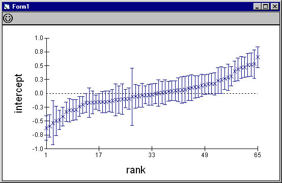
The caterpillar graph below is created from the residuals window and represents a set of ordered shrunken residual estimates of school effects with 95% confidence intervals from a variance components model.