Random intercept models

A transcript of random intercept models presentation, by Rebecca Pillinger

• To watch the presentation go to Random intercepts models - listen to voice-over with slides and subtitles (If you experience problems accessing any videos, please email info-cmm@bristol.ac.uk)

1. Random intercept models: What are they and why use them?
   
   • Explanatory variables
   • Using a single-level regression model
   • Solution: Random Intercept Model
   • Fixed and random part
   • What does the model look like?
2. Random intercept models: Research questions and interpretation
   
   • So how do we interpret the parameters?
   • Substantive interest vs. nuisance
   • Examples of research questions
3. Random intercept models: Adding more explanatory variables
   
   • Example
   • When is a variable a level?
   • Guidelines
     • Examples
4. Random intercept models: Hypothesis Testing
   
   • Likelihood ratio test
5. Random intercept models: Variance partitioning coefficients
   
   • ρ and clustering
   • Interpreting the value of ρ
   • Clustering in the model
6. Random intercept models: the correlation matrix
   
   • Assumptions of the random part
   • V, the correlation matrix
   • Covariance matrix for a single level model
   • Covariance matrix for a random intercepts model
   • Calculating the covariances
   • V for random intercepts model
7. Random intercepts models: Residuals
   
   • Multilevel residuals
   • Why do we shrink?
   • Points to note about shrinkage
8. Random intercepts models: Predictions
   
   • Visualising the model

1) Random intercept models: What are they and why use them?

Explanatory variables

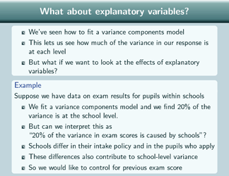
We've seen how to fit a variance components model and that lets us see how much of the variance in our response is at each level. But what if we want to look at the effects of explanatory variables?

So for example, suppose that we have data on exam results of pupils within schools and we fit a variance components model, and find that 20% of the variance is at the school level. But can we really interpret that as meaning "20% of the variance in exam scores is caused by schools"? Because schools differ in their intake policy and in the pupils who apply. So this 20% variance at the school level could actually be caused, partly or wholly, by the fact that the pupils were actually different before they entered the school. So we'd actually like to control for the previous exam score so that we can try and look at just the variance that's due to things that have happened whilst those pupils are at that school.

Using a single-level regression model

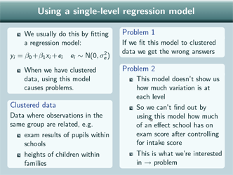
Well usually, if we want to control for something, we do that by fitting a regression model, like this, but when we have clustered data, using this single level model causes problems, as we've seen. And clustered data are data where observations in the same group are related, so, for example, exam results for pupils within schools, or heights of children within families.

So the first problem, of using this model with clustered data, is that we'll actually get the wrong answers, so for the standard errors, our estimates will actually be wrong. And we saw that a bit in the first presentation about different analysis strategies.

The second problem, is that that model doesn't actually show us how much variation is at the school level, and how much is at the pupil level. And so if we fit that model, we won't actually find out how much of an effect school has on exam score after controlling for intake score and since that's what we're interested in, that's a problem.

Solution: Random Intercept Model

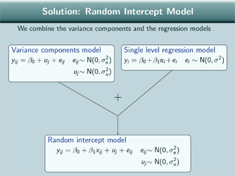
So what we do is we combine the variance components and the single level regression model and we get a random intercept model. So the random intercept model has got 2 random terms, just like the variance components model so we've got a variance of the level 1 random term here …a variance of the level 2 random term here

So we are going to be able to see how much variance is at each level. But like the single level regression model, we've included the explanatory variable so we are controlling for that.

Fixed and random part

The random intercept model has two parts. It's got a fixed part (which is the intercept and the coefficient of the explanatory variable times the explanatory variable) and it's got a random part, so that's this u_j + e_ij at the end.

So the parameters that we estimate for the fixed part are the coefficients β₀, β₁ and so on and the parameters that we estimate for the random part are the variances, σ ²_u and σ ²_e.

The random part is random in the same way that the error term of the single level regression model is random. All that means is that the u_j and the e_ij are allowed to vary so that you can think of it as being that some unmeasured processes are generating the u_j and the e_ij.

What does the model look like?

So what does the random intercept model actually look like? Well first of all let's remind ourselves of what the variance components and the single level regression model look like. So the variance components model…

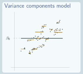
has a line for each group and all of those lines are parallel to the overall average line, and that's just a flat line, because here we plotted our data against our explanatory variable x but x hasn't actually been involved in our model so although you can see the underlying data, you can see that the underlying data have a relationship between x and y. In terms of our model which is the lines that we fitted here, there isn't any relationship between x and y because we didn't include one.

For the single level regression model, we only have one line, just one overall line, but that line isn't just flat, that line is showing the relationship between x and y.

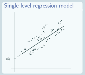
And we can colour in those graphs according to which group the points have come from.

‌

So our random intercept model now:

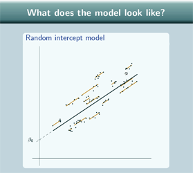
Well, like the variance components model, our random intercept model has one line for each group, and, again, they're parallel, these lines, to the overall line. Like the single level regression model, the overall line is not just flat, the overall line slopes to fit our data points so it is showing a relationship between x and y and again we can colour in the points according to which group they come from.

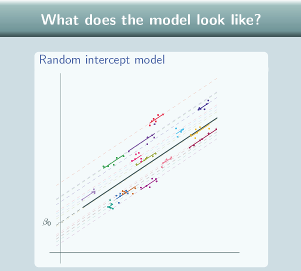
We can extend the group lines because our model equation doesn't specify the length of those lines. In theory they go on forever, but often we won't actually draw them fully extended, we'll only draw them for the range of our data.

So what does our u actually look like for this model?

Well, u is just the difference between the intercept of the overall line and the intercept of the group line so it's just this difference here: 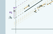and in this case we're looking at u for group 1 so it's the difference between the intercept of the overall line and the intercept for group 1. If we look now at group 7, u₇ here 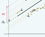is the difference between the intercept for the overall line, and the intercept for the line for group 7, this difference here.

And if we look at group 11 now 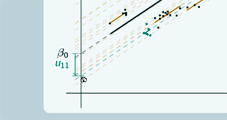For this group, the intercept of the group line is below the intercept of the overall line so u₁₁ will be negative.

Just to recap that, like the single level regression model, the overall line for the random intercept model has the equation β₀+β₁x_ij and like the variance components model, each group has its own line, and those lines are parallel to the overall average line.

So what's this random intercept? Why do we call it a random intercept? Well, for the single level regression model, the intercept is just β₀, and that's a parameter from the fixed part of the model. For the random intercept model, the intercept for the overall regression line is still β₀ but for each group line the intercept is β₀+u_j and you can see that if we go back to the graphs.

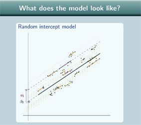
So here we have group 1, so if we want to find the intercept for group 1 we take β₀, the intercept for the overall line, and we add on u₁, so the intercept is β₀ +u₁. It's true as well when we have the negative u, so the group 11 - here's the intercept of the group line and what we do to get there is we take β₀ and we add on this negative value u₁₁ so the intercept is still β₀+u₁₁.

So this actually involves a parameter from the random part, this u_j , and so that means that this intercept is allowed to vary so we call it a random intercept. It's worth noting as well that the terminology is slightly confusing here. Sometimes we call this, , the random intercept, and sometimes we just call u_j the random intercept so you have to work out from the context which of those two is meant. But often, actually, statements about one of them are true for the other as well so it doesn't make much of a difference.

2) Random intercept models: Research questions and interpretation

[What] questions can we answer using the random intercept model? Well we can use the model to answer two kinds of question.

1. Questions about variables: So for example "What is the relationship between exam score at age 11 and exam score at age 16?" So normally we would fit just the single level regression model but we can't because we have clustering in our data. But the model, the random intercept model, has allowed for the clustering in our data, so we can now answer the question. And it's a question about means, and we answer it using the fixed part, so in this case, the slope β₁ of the overall regression line. So, just in the same way that if we had fitted a single level regression model, we'd use our estimate of β₁ to answer the question.
2. We can also answer questions about levels. So for example "How much variation in pupils' progress between age 11 and 16 is at the school level?" And that's a question that we would answer with a variance components model, but we can't do that because we need to control for the differences in intake. The random intercepts model does control for those differences, and it's a question about variances, and it's answered using the random part, we use the level 2 variance, σ ²_u

So how do we interpret the parameters?

Well, for the fixed part we can interpret the parameters just the same as for a single level regression model. So β₁ is the increase in the response for a 1 unit increase in x.

For the random part, we interpret the parameters just as for the variance components model, and again note that the parameters that we estimate are σ ²_u and σ ²_e , not u_j and e_ij , so we're interpreting the variances, not the individual school effects, just the same as for the variance components model. So σ ²_u is the unexplained variation at level 2 after we control for the explanatory variables. And σ ²_e is the unexplained variation at level 1 after we control for the explanatory variables.

Substantive Interest vs. nuisance

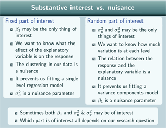
Sometimes, when we come to interpret the estimates for our random intercepts model, we may only be interested in the fixed part of the model. So β₁, for example, may be the only thing of interest. And that's when we we want to know what the effect of the explanatory variable is on the response and the clustering in our data is just a nuisance which prevents us from fitting a single-level regression model. And so in that case we can look at σ ²_u as being just a nuisance parameter. So we don't look at our estimate for σ ²_u and interpret it.

On the other hand, sometimes only the random part is of interest, so in that case σ ²_u and σ ²_e are the only things that we want to look at. And that's when we want to know how much variation is at each level and in that case the relation between the response and the explanatory variable is a nuisance. So that's like our example - when we wanted to control for intake score when looking at school exam results. So this relation between the response and the explanatory variable prevents us from fitting a variance components model. So, in this case, we might look at β₁ as being a nuisance parameter.

Sometimes, both β₁ and σ ²_u and σ ²_e may be of interest. And which part is of interest, all depends on our research question.

So here are some -

Examples of research questions

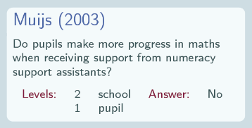
So this study [Muijs, 2003] looked at whether pupils make more progress in maths when they receive support from numeracy support assistants. So they had school at level 2 and pupil at level 1, and of course they expected that pupils within the same school would be more similar than pupils from different schools. So they had to fit the random intercept model, they couldn't fit a single level regression model, and their answer to that question was: No, pupils don't make any more progress in maths when they receive support from numeracy support assistants.

This study [Southwell, 2005] looked at whether memory of health campaign advertisements increases as extent of past drug use increases, and they were actually interested in whether the impact of the advertisements increases, and memory was what they were using to measure impact. They had advert at level 2 and individual at level 1 because each advert was seen by more than one person, and of course they expected memory of the same advert to be more similar than memory of different adverts, and their answer to the question, again, was: No, the memory of health campaign advertisements doesn't increase as the extent of past drug use increases. So they interpreted that as meaning, for individuals with more past drug use, an advertisement doesn't have any more impact than for individuals with less past drug use.

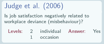
This study [Judge et al., 2006] looked at whether job satisfaction is negatively related to something they called 'workplace deviance' which is misbehaviour at work - and they were looking at individuals over time. Each individual was measured as to their workplace deviance and their job satisfaction on several days, and of course they expected that for the same person, both the job satisfaction and the misbehaviour would be more similar than for a different person so they had to fit a random intercept model, they couldn't just fit a single-level regression model. And their answer was: Yes, job satisfaction is negatively related to workplace deviance, so people who are less satisfied at work misbehave more, or, people who [mis]behave less at work are more satisfied in their job.

This study [Buckley et al., 2008] looked at whether flowering stem length was related to vegetative stem length in St John's Wort. They had quadrat at level 2 and plant at level 1. A quadrat is a sort of sampling frame, maybe a metre square and they take every plant which falls inside that sampling frame. So obviously you'd expect plants in the same sampling frame to be more similar than plants in different sampling frames. That's partly because the conditions would be more similar within that one square metre, it's more likely to have similar levels of shade and similar levels of rainfall and so on. But it's also actually because St John's Wort reproduces asexually as well as sexually, so they didn't know whether plants within the same quadrat were actually clones of each other so they had to allow for the clustering at the quadrat level, partly due to similar conditions but also due to probably similar genes in their plants. And their answer was: Yes, that flowering stem length is linked to vegetative stem length.

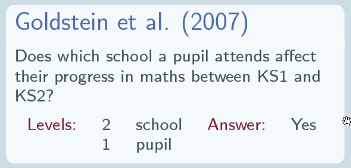
And finally, all these other 4 studies have been looking at the fixed part of the model so that for them the clustering has been a nuisance and they would have liked to have fitted a single level regression model. This study [Goldstein et al., 2007] is an example of a study for which the relationship between the explanatory variable and the response is a nuisance and they fit the random intercept model to allow for that relationship. Again, it's a case of pupils in schools and basically this is a paper giving the example that we had earlier with the response being exam score, this Key Stage 2 test, and the explanatory variable being the previous exam score, Key Stage 1. So, in that situation where the response is exam score and the explanatory variable is previous exam score, actually they're looking at progress and so they're looking at the variation in progress. So they have schools at level 2, pupils at level 1, and the answer is: Yes, which school a pupil attends does affect their progress in maths.

And here are the details of all those studies:

• Buckley, Y., Briese, D. and Rees, M. (2008) Demography and management of the invasive plant species
  Hypericum perforatum. I. Using multi-level mixed-effects models for characterizing growth, survival and
  fecundity in a long-term data set Journal of Applied Ecology, 40 pp 481 - 493
• Goldstein, H., Burgess, S. and McConnell, B. (2007) Modelling the effect of pupil mobility on school
  differences in educational achievement Journal of the Royal Statistical Society Series A, 170 4 pp 941 - 954
• Judge, T., Scott, B. and Ilies, R. (2006) Hostility, job attitudes and workplace deviance: Test of a
  multilevel model Journal of Applied Psychology 91 1 pp 126 - 138
• Muijs, D. (2003) The effectiveness of learning support assistants in improving the mathematics
  achievement of low achieving pupils in primary school Educational Research 45:3, pp 219 - 230
• Southwell, B. (2005) Between messages and people: A multilevel model of memory for television content
  Communication Research 32 1 112 - 140

3) Random intercept models: Adding more explanatory variables

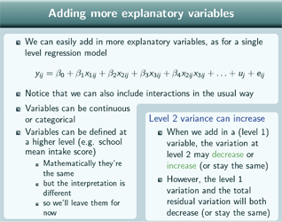
So far we've looked at examples of random intercept models with only one explanatory variable but in fact we can easily add in more explanatory variables, just in the same way as for a single level regression model. So, we've got an example of that here where we've got another couple of explanatory variables added in. And interactions, we can also add in, in exactly the same way as for a single level model. Variables can be continuous or categorical. Of course, if we have a categorical variable we enter that as a set of dummy variables, just as for a single level regression model. And variables can be defined at a higher level. So, for example, school mean intake score, we say that's defined at a higher level because the school mean intake score will take the same value for every pupil within that school. Pupils in the same school will have the same value of this variable. Now mathematically, that's exactly the same. It goes into the model exactly the same and it goes into MLwiN in exactly the same way but the interpretation of these variables is different and so we're going to leave those for now and only look at variables defined at level 1.

Now when we put in explanatory variables, the level 2 variance can increase. Now we're used to the idea with single level regression models that when you put in an explanatory variable the variance goes down. For a random intercept model it's true that the level 1 variation and the total residual variation will both decrease when we put in an explanatory variable. But the level 2 variance can increase, and that's true not only when we add in a second explanatory variable, but actually also when we add in the first explanatory variable, to go from the variance components model to the random intercepts model.

Example

So as an example of that let's look at modelling house prices. So in this case, area is level 2 and house is level 1. So we start with a variance components model and then we add in house size as an explanatory variable. And actually more expensive areas tend to have smaller houses. For example, in London the expensive areas tend to be in the centre of the town where there's not so much room for larger houses. Because the more expensive areas have smaller houses, that means that in the variance components model, before we add in house size, the fact that the houses are smaller is bringing down the average price for those more expensive areas so they don't appear as much more expensive. And similarly for the less expensive areas, which tend to have larger houses, before we add in house size, the average price for that area is brought up by the fact that the houses in that area are larger. So that means that before we add size, the house prices will appear more similar across areas and after we add size, the average price for the expensive areas is no longer being brought down because we've adjusted for the size and the house price for the less expensive areas is no longer being brought up, because we've adjusted for the size.

So the variance components model will have less variation at level 2 because the areas appear more similar than the random intercept model.

When is a variable a level?

So when we come to adding in more explanatory variables, we may wonder: When should we add in an explanatory variable as an explanatory variable and when instead should we put it in as a level? Because, for example, when we have our example of pupils within schools, we could have put in school as a fixed explanatory variable, and allowed each school to have a different effect in the fixed part of the model but we decided not to do that, we decided to put school in as a level, but, you know, the question comes up with many other explanatory variables: Should we put it in as an explanatory variable or should we put it in as a level? Well, it's not an easy question. Sometimes, it is very clear cut. Sometimes we wouldn't consider using a variable as a level, we would definitely put it in as an explanatory variable, and sometimes we definitely would want to put it in as a level, we definitely would not put it in as an explanatory variable. But often, it's less obvious what we should do, and it's often when we have a relatively small number of units, which would be at that level if we put it in, when it's less obvious what we should do. So, for example, if we are considering: Should we put in country as a level or as an explanatory variable and we might only have a few countries, so is that enough? Basically two things govern our decision about what to do, one is the number of units and the other is exchangeability.

Exchangeability: The units are exchangeable if we could randomly reassign their codes without losing any information. So that's quite a complicated concept to understand, so we're going to give some guidelines.

The units basically should be a representative draw from the population, so that's why these 2 things - number of units and exchangeability, are important, because obviously if we don't have enough units, then they will not be a representative draw, and if we don't have exchangeability, that means that we're not drawing from a population. And, as we've said, exchangeability is a tricky concept, so we're going to give some guidelines.

Guidelines

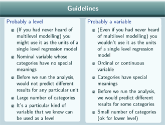
These basically take into account both those points about number of units and about exchangeability. So a kind of overall guideline is: If you had never heard of multilevel modelling, might you use this variable as the units of a single level regression model? So in our example of schools, if you had never heard of multilevel modelling, you might decide that the best way to analyse your data for pupils within schools would be to take averages for each school of both your response and your explanatory variables, and then have those averages as your data points and fit a single level regression model to those. Of course now we know that this is not a sensible thing to do because we have been learning about multilevel modelling and we know that that will give you the wrong standard errors. But since, if you hadn't heard of multilevel modelling you might do that, that implies that school is probably a level, you probably can use it as the level 2 units in a multilevel model. On the other hand, if you ask that question for something like gender, then, even if you had never heard of multilevel modelling, you would not take the average for men and the average for women and then fit a single level regression model to those 2 data points. So that suggests that, for gender, we don't want to put that in as a level, we should put it in as a variable.

Here are some other guidelines which actually explain why we might answer either way to these question, that kind of break this down a bit.

If we have a nominal variable whose categories have no special meanings, so that's like school for example. School 63 doesn't have a special meaning compared to school 111, it really doesn't matter which school gets which of those categories. So in that case, the variable can probably be put in as a level. But on the other hand, if we have an ordinal or continuous variable, so something like income bands, or just income measured as a continuous variable, then we'd probably have to put that in as a variable, not as a level. Or if our categories have special meanings, like with gender, male and female have special meanings and if we swap those labels around, then, when we try to interpret our estimates, we'll be looking at the wrong thing. In that case, the categories do have special meanings and so if that's true, we probably don't want to put that in as a level, we want to put it in as a variable.

Also, if, before we run the analysis, we wouldn't predict different results for any particular unit, then we can probably put it in as a level. So with the schools for example, before we run the analysis we have no reason to believe that any particular school will have a greater effect than any other. If we did, then that would mean that we would probably have to take that school out and put it in the fixed part of the model. If, before we run the analysis, we would predict different results for some categories, so like with gender, we'd predict different results for men and women, and we can probably guess which way round, whether we'll have a greater estimate for women or for men, we probably can't put that in as a level, we probably have to put that in as a variable.

And then there's the number of categories, so for school we have a large number of categories so it's probably OK to put that in as a level, but for gender, we have a small number of categories, just two categories, so we probably can't put that in - at level 2. It is important to note that the number of categories doesn't matter for lower levels, it's only the highest level, that the number of categories matters in this decision.

And finally, if it's a particular kind of variable that we know can be used as a level, then, even if it appears to violate some of these conditions, then it's still OK. Examples would be repeated measures, so when we've got several time occasions, that would be an example of a variable that is ordinal, but we can find out from textbooks and courses that we can use that variable as a level so we can put that in.

So, some examples to understand how to do this:

Well, hospital is probably a level. Suppose that we have data on treatment outcomes for patients in 100 UK hospitals. Now, if we didn't know about multilevel modelling we might naively use the hospitals as units in a single level model. We might take the average for each hospital of the response and the explanatory variables and fit a single level model to those data points. Also, hospital ID is a nominal variable whose categories have no special meanings. Hospital 28 is no different from hospital 163, as a category name, it doesn't mean anything special, and we wouldn't expect any particular hospital to give different results, before we run the analysis.

Ethnicity, on the other hand, is not a level, if we have data on height for people of a variety of ethnicities. Even if we could measure ethnicity very finely, using many categories, even if we could measure ethnicity using 50 categories, say, we still wouldn't use it as the units in a single level model. We wouldn't take the average for each ethnicity and fit a single level regression model to those points and that's because the categories of ethnicity have a special meaning. Black has a special meaning compared to Asian, and we do expect different results for different categories. In the case of height we might expect Asian (and if we have sub-categories of Asian those sub-categories) to have smaller values of height than some of the other ethnicities. And in any case, the idea that we might be able to measure ethnicity by 50 categories is probably unrealistic. Probably we don't have very many ethnicity categories, we may only have 6 categories, say. So for these reasons we can't put ethnicity in as a level.

4) Random intercept models: Hypothesis Testing

‌

[Hypothesis] testing is of course an important part of interpretation because we don't only want to know the size of the fixed effects and the amount of variance at each level, we also want to know whether the fixed effects are significant and whether there's a significant amount of variance at level 2.

For the fixed part, hypothesis testing is just the same as for a single level model. We just divide the coefficient by its standard error, to get z, and then we take the modulus of z, and if that's bigger than 1.96 (or informally we can use 2) then β₁ is significant at the 5% level.

For the random part we can't just divide σ ²_u by its standard error and compare the modulus with 1.96. Instead, we have to fit the model with and without u_j and do a likelihood ratio test comparing those 2 models, to see whether σ ²_u is significant.

Likelihood ratio test

So here are the two models that we fit, This one has u_j :

and this one doesn't have u_j:

So this is our random intercept model:

and this is a single level regression model:

which is exactly the same in terms of the explanatory variables. The only difference is that it doesn't have u_j. So we fit those and we note the likelihoods. The test statistic is 2 times the log of the likelihood of the random intercept model minus the log of the likelihood of the single level regression model:

And MLwiN, in fact, gives minus 2 times the log likelihood in the Equations window so if we're using MLwiN, then we can just take MLwiN's value for the single level model and subtract MLwiN's value for the random intercepts model:

The null hypothesis is that σ ²_u = 0. and if that's true then we don't need u_j in the model so we can just fit the single level regression model . So we compare the test statistic to the distribution with 1 degree of freedom. And then we can divide the corresponding p-value by 2 since σ ²_u has to greater than or equal to 0.

There is one degree of freedom because there is one more parameter, σ ²_u , in the random intercept model, compared to the single level regression model.

5) Random intercept models: Variance partitioning coefficients

So when we were looking at variance components models, we found that the variance partitioning coefficient is a useful way to see how the variance divides up between levels. And it's actually even more true for random intercept models because, as we saw earlier, the total amount of variance may change as we add explanatory variables, which can make comparison hard.

It's important to note, in what we're about to say, that we most often use level 1 variance to mean residual variance at level 1, not the variance of y at level 1 and the same thing for level 2 variance.

So how do we calculate the variance partitioning coefficient? Well, remember that the variance partitioning coefficient is the level 2 variance divided by the total residual variance. And for a random intercept model, our level 1 variance is σ ²_e , our level 2 variance is
σ ²_u
and the total residual variance is σ ²_e + σ ²_u . So our variance partitioning coefficient is σ ²_e over σ ²_u + σ ²_e and that's just exactly the same as for the variance components model.

ρ and clustering

Another way to think of ρ is that it measures the clustering.

If we have a large value of ρ then a lot of the variance is at level 2 and that means that units within each group are quite similar but that there's a lot of difference between groups and so values of the response are largely determined by which group the unit belongs to, and so the data are very clustered.

If we have a small value of ρ then not much variance is at level 2, and so units within each group may be quite dissimilar but there's not much difference between groups. So which group a unit belongs to, doesn't have much of an impact on the response and the data are not very clustered.

So here's an example of a graph for a particular value of ρ:

‌

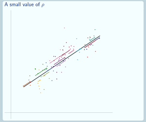
Is this a graph where we have a large value of ρ or where we have a small value of ρ? Well, this is a small value of ρ because in this case, there's not much variation in the group lines, but there's quite a bit of variation in the individual data points around their group lines.

Here's an example of a different value of ρ:

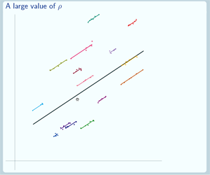
Is this a small value of ρ or a large value of ρ? Well, this is a large value of ρ because in this case there's a lot of variation of the group lines around the overall line but not much variation of the individual data points around their group lines.

So in theory, ρ can actually be as large as 1 or as small as 0 - so what do those values actually look like? Well here's one of them: Is this ρ =1 or ρ =0?

‌

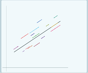
Well this is ρ =1. In this case, there's no variation at level 1. There's variation at level 2 because the group lines vary round the overall regression line but there's no variation at level 1 because the individual data points don't vary around their group lines. So in this case, we have complete dependency. If we know the value of the explanatory variable and we know which group a data point belongs to, then we know the value of the response for that data point. And obviously, that doesn't really tend to happen in practice in the social sciences.

Now if we want to look at ρ =0 (we'll build it up gradually so it's easier to see):

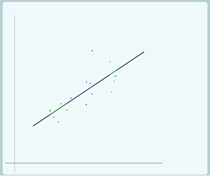
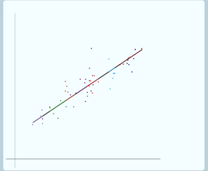
In this case, there's no variation at level 2 so the group lines don't vary around the overall regression line, all of the group lines lie on the overall regression line. But the individual data points do still vary around their group line, still have level 1 variance.

Interpreting the value of ρ

If we look at the formula for p, as we said, we can see that in theory the smallest it can be is 0. So in this case when ρ is 0 we don't have any dependency. If we know the value of the explanatory variable for a data point then knowing which group it comes from doesn't tell us anything more about its value of the response. In this particular example, we do have dependency in terms of x. You can see that for the yellow group here,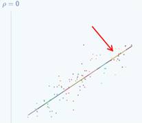
all of the data points have quite high values of x

whereas for the green group here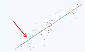
all of the data points have quite low values of x

So in terms of x there is dependency. But we're interested in whether there's dependency in y after controlling for x and there isn't any dependency there. So in this case, we could actually use a single level regression model.

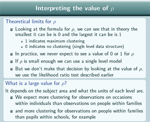
So as we just said, if we look at the formula for ρ we can see that, in theory, the smallest ρ can be is 0 and the largest it can be is 1 and 1 indicates maximum clustering and 0 indicates no clustering. So it's basically a single level data structure. In practice, though, we never expect to see a value of 0 or 1 for ρ. If ρ is small enough, we can use a single level model but ρ doesn't have to be 0, just small enough. But we don't make that decision by looking at the value of ρ, we do that by testing the significance of σ ²_u in our random intercepts model using the likelihood ratio test which we described in the section on hypothesis testing.

So, OK, in practice we're not going to see a value of 1 for p. What is a large value? Well, that actually depends on the subject area, and on what the units of each level are. If we have observations on occasions within individuals we expect quite a lot of clustering but we expect less clustering for observations on people within families and we expect less clustering again for observations on pupils within schools. And for a more detailed presentation of ρ and dependency you can see the audio presentation Measuring Dependency which is also on our web site.

Clustering in the model

So we've talked a lot about clustering in the previous presentations. Clustering was the reason why we can't use a single level regression model. It's why we have variance at both level 1 and level 2 - so why our response is actually determined at two levels. We've seen how to measure the clustering and how to interpret it.

But what we haven't seen yet, is how the clustering is incorporated into the model, why it is that the random intercept model can allow for the clustering but the single level model can't. So how does the random intercepts model actually allow for similarities between different observations from the same group? Well, to discover this we need to look at the correlation matrix, V and in order to do that we're going to need to return to the technicalities of the model.

6) Random intercept models: the correlation matrix

Assumptions of the random part

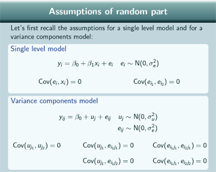
So, first of all, let's recall the assumptions for a single level model and for a variance components model.

For the single level model we assume that the residual and the covariantes are uncorrelated and that 2 different residuals are uncorrelated.

For the variance components model we assume that the level 2 residuals for 2 different groups are uncorrelated, that the level 1 and the level 2 residuals are uncorrelated, whether from the same or a different group and that 2 different level 1 residuals are uncorrelated, again whether from the same or from a different group.

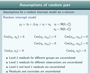
For the random intercept model, we have a mixture of assumptions from the single level and from the variance components model. We again assume that the level 2 residuals for different groups are uncorrelated and we assume that the level 2 and the level 1 residuals are uncorrelated. We assume that the level 1 residuals for different observations are uncorrelated and we assume that residuals and covariantes are uncorrelated.

V, the correlation matrix

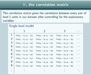
The correlation matrix gives the correlation between every pair of level 1 units in our dataset after controlling for the explanatory variables. The columns - each column is one individual in our dataset and each row is also one individual in our dataset.

So here's the correlation of individual 1 with themselves: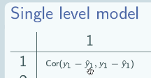

Here's the correlation between individual 1 and individual 2: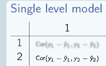

Here's the correlation between individual 2 and individual 9: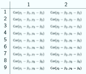

And so this matrix extends towards the right, it extends downwards as well, it basically covers our entire dataset. The correlations that we're taking, what we do is we take away the fixed part of our model and we take the correlation between what's left so the correlation between the random parts of the model, because that will be the correlation after controlling for the explanatory variables.

So how do we actually work out what these correlations come to?

Well first of all, note that, for the single level model, this here - - is just going to be just e_i , the one random term. So what the correlations were actually trying to calculate are just these - - the correlation between the level 1 residual for each pair of individuals. The other thing to remember is that the correlation is the covariance divided by the total variance so the easiest way to work out the entries of this matrix is to calculate the covariance matrix and then divide all of the terms by the total variance which will give us the correlation matrix.

So to calculate the covariances, we need two things, one of them is this handy rule - - which says that the covariance of something with itself is just the variance of that thing. And the other is all the assumptions that we've just seen.

Covariance matrix for a single level model

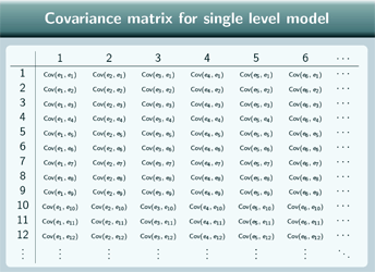
So the covariance matrix for the single level model is this, basically we're just taking the covariance of these terms.

‌

For the same observation - that's all the diagonal terms - the covariance of each level 1 residual with itself is just the variance and we define that to be σ ²_e so all the diagonal terms are
σ ²_e.

Two different observations, the covariance is 0 because that was one of our assumptions.

So here's the covariance matrix for a single level model:

‌

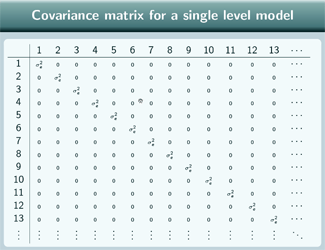
σ ²_e down the diagonal, and 0 everywhere else and the total variance for the single level model is just σ ²_e so we divide by that and get 1s down the diagonal and 0s everywhere else. This shows us that for this single level model, of course each individual - the correlation with themselves is 1 - but any pair of different individuals, their random terms are uncorrelated. So, after we've controlled for the explanatory variables, there's no correlation between a pair of different individuals if we use the single level model.

Covariance matrix for a random intercepts model

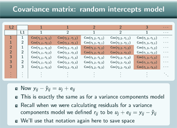
So, moving onto the random intercepts model now - now we've got a more complicated data structure we've got actually level 1 units within level 2 units so, for example, pupils within schools.

(L2 = 1, L1 = 1) So now this is pupil 1 within school 1, (L2 = 1, L1 = 2) this is pupil 2 within school 1. (L2 = 2, L1 = 1) Here's pupil 1 within school 2, (L2 = 2, L1 = 2) pupil 2 within school 2, (L2 = 3, L1 = 1) pupil 1 within school 3.
And the same for the rows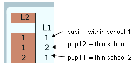

(L2 = 1, L1 = 1) pupil 1 within school 1, (L2 = 1, L1 = 2) pupil 2 within school 1, (L2 = 2, L1 = 1) pupil 1 within school 2, …and so on.

Obviously this is just a reduced example so it will all fit on the screen, obviously really we'd expect to have more pupils per school.

For the random intercept model, this thing that we're taking the covariance of, is just u_j + e_ij and we've actually written this here as r_ij because, if you remember, in the variance components model, when we were calculating residuals we actually defined r_ij to be just u_j + e_ij. So we've written that here because it takes less space basically. And this covariance matrix is just the same as for a variance components model, if we were taking the covariance matrix for a variance components model we'd have exactly the same thing to calculate.

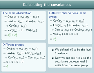
Calculating the covariances

When we're calculating these covariances, for the same observation, this is what we get, and we won't go into the details but that comes out as the Variance of u_j +0+Variance of e_ij so these are just - the variance of u_j is just defined to be σ ²_u and the Var of e_ij is defined to be σ ²_e . For the same individual (on the diagonal terms) you have σ ²_u + σ ²_e . For 2 individuals from different groups, this covariance comes out to be this:

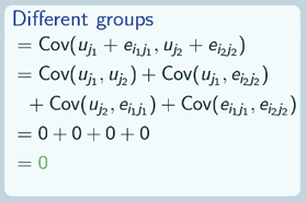
and all of these are things that we assumed were 0 when we were looking at the assumptions of the model. So for 2 individuals from different groups, we just have a covariance of 0.

For 2 different individuals from the same group, the covariance comes out to be this:

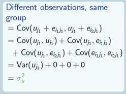
and these 3 terms we assumed were 0 but this one -
- is the variance of u_j and we defined that to be σ ²_u so for 2 different observations from the same group we have σ ²_u as the covariance.

Now it might seem a bit strange - we introduced σ ²_u at the beginning when we were looking at the variance components model for the first time - we introduced that as the level 2 variance and now we're saying - it's the covariance between level 1 units from the same group. Actually if you think about it, it's not that strange that those two things would be equal because the differences between groups are kind of the similarities within groups, it's just two different ways of looking at the same thing really.

Here's our covariance matrix with all the terms filled in, so we've got σ ²_u+ σ ²_e down the diagonal so for each individual the covariance with themselves is the total variance and for 2 different individuals from the same group we've got σ ²_u and for 2 individuals from different groups we've got zero covariance.

So we now divide through by the total variance σ ²_u + σ ²_e so we can get the correlation matrix so for the diagonal terms that will just become 1. For 2 individuals from different groups that will be 0 still and for 2 individuals from the same group, 2 different individuals from the same group, that will come out to be the variance partition coefficient, ρ. So that's why, as we saw with the variance components model, the intra-class correlation is the same as the variance partitioning coefficient.

V for random intercepts model

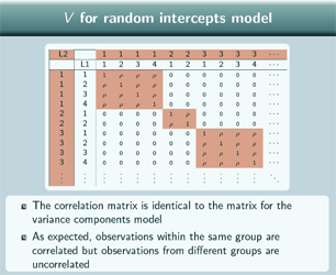
The correlation matrix shows us that for the random intercepts model and the variance components model (because that has the same correlation matrix) 2 individuals from different groups are uncorrelated after we control for the explanatory variables but 2 individuals from the same group, after we control for the explanatory variables, have correlation ρ. So that shows how the random intercepts model is allowing for that correlation between different observations from the same group.

7) Random intercepts models: Residuals

So, having looked at the correlation between the residuals, let's look at the residuals themselves in a bit more detail.

The residuals are estimates for the random part. For a single level model we often say estimates for the error term. And just a quick reminder - for a single level model - the residual for an observation is an estimate for e_i so we've got here an estimate for ê₅₄ and an estimate for ê₄₄ here and if we write - - then our estimate for our residual is the observed value of y minus . It's the observed value minus the value predicted by the regression line. So that's what we can see here, the estimate for the residual is the distance between the data point and the overall regression line.

Why are we actually interested in the residuals?

Well often we're not, but they can be useful in some cases.

So one example is diagnostics. We can plot the residuals to check their normality and that's part of checking how well the model fits.

We can also rank level 2 units by their level 2 residuals and an example of that is school league tables.

Sometimes we're interested in a particular unit, we want to find out how that particular unit compares to the average.

And then we need the level 2 residuals in order to make predictions for individuals in a particular level 2 unit and we need them in fact to graph the group lines which are the predicted lines for each group.

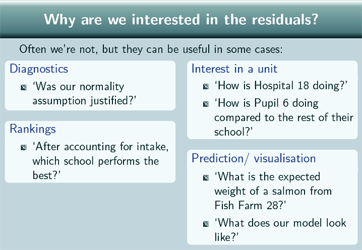
A few examples of those uses:

For the use of diagnostics we might be asking "Was our normality assumption justified?"

For rankings we might be asking "After accounting for intake, which school performs the best?"

For interest in a unit, we might be asking "How is Hospital 18 doing?" or: "How is Pupil 6 doing compared to the rest of their school?"

And in terms of prediction and visualisation, we might be asking "What is the expected weight of salmon from Fish Farm number 28?" or "What does our model look like?"

Multilevel residuals

‌

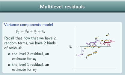
So just recall briefly that for the variance components model, because we have 2 random terms, we have 2 kinds of residual. We've got the level 2 residual, which is an estimate for u_j , and the level 1 residual which is an estimate for e_ij.

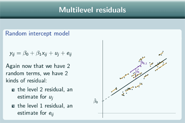
And for the random intercept model, again, now that we have 2 random terms, we have 2 kinds of residual, again an estimate for u_j and an estimate for e_ij.

And the calculation is very similar too for the variance components model:

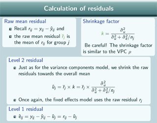
Remember that we have the raw mean residual, which is the mean of r_ij, for group j, and r_ij is just the datapoint minus the value predicted by the overall regression line.

And we have the shrinkage factor again with the same formula as for the variance components model - and again we need to be careful because the shrinkage factor is quite similar to the VPC, the variance partitioning coefficient p, so it's important not to get those confused.

So the level 2 residual is calculated in just the same way as for the variance components model. We take the raw mean residual and multiply by the shrinkage factor. Once again, if we have the fixed effects model then we wouldn't shrink the residual, we'd just use the raw residual, but for the multilevel models, for the variance components model and for the random intercept model, we do shrink the residual.

Level 1 residual is simpler, we just take the observed value and subtract the value predicted by the overall regression line and the level 2 residual, so that's just the raw mean residual minus the level 2 residual.

So why do we actually shrink?

Well, in order to explain that, let's do a thought experiment. So imagine that we have exam results for 6 pupils each from a number of schools and suppose that we drop 4 pupils from 1 school just to see what will happen. If we do that, how close will the school line using the remaining 2 pupils be to the correct line using all 6 pupils?

Well, that will depend on how typical those 2 pupils are of the full set of 6. Because we are picking 2 pupils from 6 it is quite likely that we might pick 2 untypical pupils and then the school line drawn using those 2 will be quite far from the school line using all 6 pupils.

And if we draw a graph of our particular example because that happens in this case:

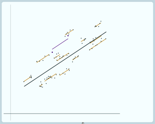
Here's the school where we have dropped 4 pupils,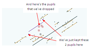

We've drawn the line here using just the 2 pupils that we kept and we can put on, again, the line drawn using all 6 pupils, you can see there's quite a gap between those 2 lines: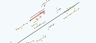

Well, we're interested, in fact, in drawing the line for all 6 pupils -

‌

it's much more interesting to know where the line for all 6 pupils is than the line for just those 2 pupils because we're interested in the school effect rather than the school effect for those particular 2 pupils. So we want our line - when we have 2 pupils - to stay close to the line for all 6 pupils and we don't want it to move around a lot depending on which 2 pupils we pick. How can we actually draw a line that does those things?

We need some information about the 4 pupils that we dropped and it seems as though we don't have any but actually that's not true. The position of the other school lines tells us something about where the 4 pupils and the line for this school are likely to be because they're more likely to be closer to the overall average line. If those 4 pupils that we dropped were further away from the overall average line than the pupils we kept they'd be going towards the direction of being outliers. But, if they're closer to the overall average line, then they're more in line with the whole distribution of schools so it's more likely that they're closer to the overall average line. So we can improve our positioning of the line by shrinking it in towards the overall average. So let's see that:

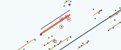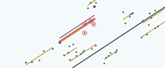So here's the line as we draw it just using those two pupils …Let's do that again, so here's where we draw it using just those two pupils	and if we now shrink it towards the overall average, this is is where it ends up …and if we shrink it towards the overall average here's where it ends up

So obviously, in our thought experiment situation, we don't know where those four pupils were, we don't know where that group line is. So if we want to do that in terms of how it looks to us, given the information available to us, here's the group line drawn just using those two pupils…

…before we shrink …here it is before we shrink	and after we shrink here it is …and here it is after we shrink.

So you might wonder: Is shrinking actually always better?

Well it is possible, that when we shrink, we will move the line away from the line using all pupils because those other 4 pupils could have been further from the overall average line so it's possible when we move towards the overall average line we are moving further away from them. But we actually don't know where the other 4 pupils are so we don't know whether shrinking will move the line closer or further away. However, we do know that shrinking will move the line closer more often than it will move it further away. And that means that shrinking the line is always our best chance to get the line closer. Shrinking the line is our best estimate. It might put our line further from the group line using all the points but our best estimate is to shrink the line and move it closer to the overall average line.

So OK, that was our thought experiment, but how does it actually generalise? Well we're actually in the same situation with our dataset as a whole. We have just 6 pupils from each school. and there are really many more. There might be 500 or 1,000 pupils in the entire school. The position of the other school lines gives us information about the likely position of the pupils not included in the dataset. So that means that, again, we'll get a better estimate of the group line by shrinking it in towards the overall average.

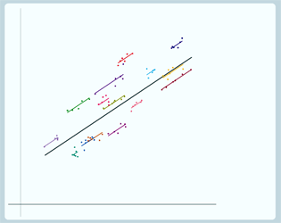
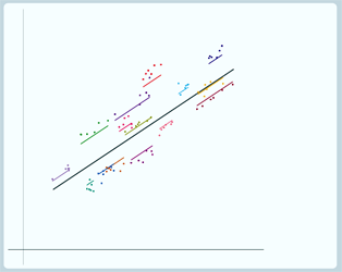
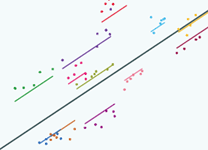
So here are our group lines drawn using just the information from the pupils in each school and if we now use the information from the pupils in all schools to draw each line by shrinking towards the overall average - here's what we get:

Let's see that again, so here's the lines before we shrink	…and here's the lines after we shrink

A couple of important points to note about shrinkage

When do we shrink? Well, we always shrink, and that's because we always have a sample from each level 2 unit. Even if we have 499 out of 500 pupils attending the school, that's still a sample. Even if we have all the pupils attending all the schools in the UK, we can still think of that as a sample from the super-population, our actual population of UK schools is a realisation from the super-population of all possible UK schools.

How much do we actually shrink by? Well, remember from the variance components model, we don't shrink by a fixed amount. If we have 500 pupils from a school we shrink less than if we have 7. Remember that the amount we shrink by depends on the absolute number of level 1 units, not the proportion of the total for that level 2 unit. If we have 10 pupils from a school then we shrink by the same amount, whether that school actually only has 10 pupils, or whether that school really has 500 pupils. We can also see that the amount of shrinkage will depend on the variances σ ²_u and σ ²_e.

And for more about the residuals and shrinkage - for a more detailed examination of the same topic - you can listen to our audio-visual presentation on residuals which is also available from the web site.

8) Random intercepts models: Predictions

Let's look at making predictions for the random intercept model now.

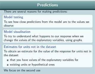
And there are several reasons why we might want to do that.

One of them is model testing. So if we want to see how close predictions from the model are to values that we actually observe, we might want to make some predictions.

Another is model visualisation. If we want to try and understand what happens to our response when we change the values of the explanatory variables then we might want to draw graphs of predicted values.

And the third reason is estimates for units not in our dataset. This would be estimates for units for which we have values of the explanatory variables and it can either be existing units that we actually have measurements on or it can be hypothetical units. And we're actually going to focus just on the second use in this section, we're only going to consider model visualisation.

Visualising the model

This idea should already be familiar from single level regression models because when we visualise a single level model we just plot  to get our graph of the overall regression line and this is just plotting the fixed part prediction, just our predicted value for the single level model. And we can add on the actual data points as well.

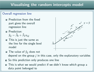
So for the random intercepts model, if we predict from the fixed part, again we get the overall regression line. So the prediction is just the same as for the single level regression model and the graph looks the same. The value of our prediction doesn't depend on group in this case. There's no difference in what this comes to depending on which group we're looking at so we only have one line produced by this prediction. And this is what we'd predict if we didn't know which group a data point belonged to. Again we can put the data points on.

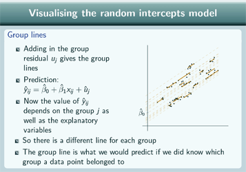
The group lines - we get by adding in the group residual to the fixed part prediction so now this is our prediction. And the value of this does depend on which group because this estimated u_j is different for every group - and incidentally you can see here how the residuals come into the prediction - because this is our level 2 residual.

So we've got a different line for each group because our predicted value depends on our group, and the group line is what we'd predict if we knew which group a data point belongs to. And again we can put on the data points.

We can combine the predictions from the fixed and random part into one graph to get a complete visualisation of the model and we can add on the actual data points for comparison. And usually we only draw our group lines for the range of values that we have in our dataset.

So here's a picture of our random intercept model: